Pre-Norm vs. Post-Norm: The Identity Path That Stabilizes LLMs
Why normalization placement changes gradient flow — with a runnable JAX stress test
The central idea: Pre-Norm matters because every Transformer block retains a residual route that normalization does not transform. That direct identity path lets gradients cross many layers. It mainly improves the optimization stability of deep models; it does not imply that Pre-Norm always has greater final expressive power.
The one-line difference
Let \(F_l\) denote either attention or the feed-forward network, and let \(N\) denote LayerNorm or RMSNorm. The two arrangements differ by one line:
Pre-Norm
\[x_{l+1}=x_l+F_l(N(x_l))\]Post-Norm
\[x_{l+1}=N(x_l+F_l(x_l))\]In Pre-Norm, only the branch computation sees normalized input. The residual stream \(x_l\) reaches the next layer unchanged. In Post-Norm, the residual is still present, but the sum must pass through normalization before becoming \(x_{l+1}\).
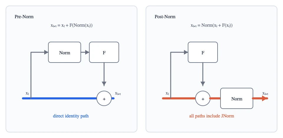
This diagram is the argument in its most useful form: Pre-Norm has an unmodified blue highway through depth. Post-Norm has a residual connection, but no unmodified identity highway.
Why the identity path changes backpropagation
Differentiate one block. Pre-Norm gives
\[\frac{\partial x_{l+1}}{\partial x_l} =I+J_{F_l}J_N.\]The \(I\) term is explicit. When the learned branch is small, as it often is near initialization, the block Jacobian is close to identity:
\[\frac{\partial x_{l+1}}{\partial x_l}\approx I.\]A gradient can therefore travel through dozens of blocks without depending entirely on the attention, MLP, or normalization Jacobians.
Post-Norm instead gives
\[\frac{\partial x_{l+1}}{\partial x_l} =J_N(I+J_{F_l}).\]Every backward route includes \(J_N\). Across a deep stack, the gradient repeatedly encounters those normalization Jacobians. Their products can rescale and rotate it, and LayerNorm projects out particular shift and scale directions. The residual addition has not disappeared; what disappeared is the untransformed identity route.
That distinction is more precise than saying “Post-Norm cuts the residual connection.” It does not. It makes normalization unavoidable on the path between successive residual states.
What Xiong et al. actually established
Xiong et al. (2020), On Layer Normalization in the Transformer Architecture, analyzed the models at initialization using mean-field arguments. Their key observation was a layerwise imbalance:
- In Post-LN, parameter gradients near the output are large at initialization. Applying the full target learning rate immediately can make the first updates unstable.
- In Pre-LN, gradient magnitudes are better behaved across depth, so their translation and BERT experiments could train without learning-rate warmup.
This explains why learning-rate warmup is especially important for classical Post-Norm Transformers: warmup makes the early updates small while the optimizer and network leave the fragile initialization regime.
Two qualifications matter:
- This is an analysis of initialization under simplifying assumptions, not a theorem that every Post-Norm run diverges.
- Modern Pre-Norm LLM training still commonly uses warmup. Warmup also helps adaptive-optimizer state, large batches, mixed precision, and other parts of the training system.
The defensible claim is therefore “Pre-Norm is less sensitive and easier to optimize deeply,” not “Pre-Norm never needs warmup.”
A runnable stability stress test
The code accompanying this article trains the same small 12-layer causal Transformer three ways:
- Pre-Norm at a constant learning rate of \(2\times10^{-3}\);
- Post-Norm at the same constant learning rate;
- Post-Norm with a linear warmup lasting two thirds of the run (120 steps in the default 180-step experiment) to the same target rate.
Everything else—data, initialization seed, optimizer, depth, width, and number of updates—is held fixed. The task is deliberately simple: given an arithmetic token sequence, predict the next token. There is no gradient clipping.
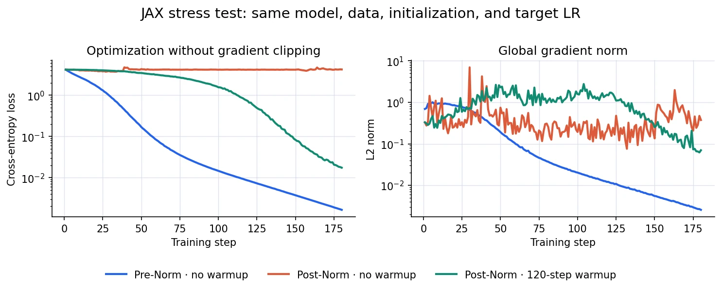
On my CPU run, the results were:
| Configuration | Final loss | Maximum global gradient norm |
|---|---|---|
| Pre-Norm, no warmup | 0.00165 | 1.004 |
| Post-Norm, no warmup | 4.21205 | 6.960 |
| Post-Norm, 120-step warmup | 0.01738 | 2.759 |
The result is intentionally not “Post-Norm is incapable of learning.” Warmup rescues it. The result is that Pre-Norm tolerates the aggressive target learning rate immediately, while this particular Post-Norm run does not.
This is a pedagogical stress test, not a reproduction of Xiong et al.: the dataset is synthetic, the model is tiny, and a different seed or hyperparameter can move the stability boundary. The useful exercise is to sweep --layers and the learning rate and observe how much tuning each topology needs.
Run it with JAX on CPU or GPU
The complete script lives beside this article:
From the repository root:
# CPU, including Apple Silicon. The full run takes about 26 seconds here.
python -m pip install --upgrade jax flax optax matplotlib pillow
python _posts/pre_norm_vs_post_norm_demo.py --device cpu

# NVIDIA GPU on Linux with JAX's CUDA 13 wheel.
python -m pip install --upgrade "jax[cuda13]" flax optax matplotlib pillow
python _posts/pre_norm_vs_post_norm_demo.py --device gpu

# Prefer a JAX GPU backend when present, otherwise use CPU.
python _posts/pre_norm_vs_post_norm_demo.py --device auto
The script writes both img/pre-vs-post-norm-stability.webp and the underlying CSV. It is JAX end to end: the model is written with Flax, gradients come from jax.value_and_grad, updates come from Optax, and the training step is compiled with jax.jit. On macOS, the supported default is Apple Silicon CPU; the JAX project does not currently ship an official macOS GPU backend. The architectural switch itself is only this:
if self.pre_norm:
    x = x + attention(attention_norm(x))
    return x + mlp(mlp_norm(x))

x = attention_norm(x + attention(x))
return mlp_norm(x + mlp(x))
The compiled update is likewise ordinary JAX:
loss, gradients = jax.value_and_grad(loss_fn)(params)
updates, optimizer_state = optimizer.update(gradients, optimizer_state, params)
params = optax.apply_updates(params, updates)
The full default run is already small enough for CPU use. For a faster smoke test, reduce the work:
python _posts/pre_norm_vs_post_norm_demo.py \
  --device cpu --layers 6 --steps 30
That shorter setting checks that the program and selected backend work; it is not guaranteed to reproduce the full stability separation.
Why Pre-Norm is not simply “better”
Pre-Norm buys optimization stability by leaving the residual stream itself unconstrained inside the stack. Expanding the recurrence shows the trade-off:
\[x_L=x_0+\sum_{l=0}^{L-1}F_l(N(x_l)).\]Every layer writes directly into the same accumulating stream. As \(\lVert x_l\rVert\) grows, a new update can become a smaller fraction of the existing state. Later blocks can approach identity transformations and contribute less than their depth suggests. Later work describes related symptoms as representation collapse, residual-stream growth, massive activations, or the “curse of depth.” The exact growth law depends on initialization, training, correlations, and residual scaling; it is not universally exponential.
Post-Norm has the opposite appeal: it re-normalizes the state after every residual addition, tightly controlling forward scale. Its cost is making normalization unavoidable in backpropagation. That is why several newer architectures try to keep the best property of each design rather than treating either as universally optimal:
| Design | What it tries to preserve |
|---|---|
| Pre-Norm | Clean identity path and robust optimization |
| Post-Norm | Controlled block-output scale |
| DeepNorm / residual scaling | Post-Norm quality with bounded updates |
| NormFormer | More balanced layerwise gradients in Pre-Norm |
| Peri-LN / sandwich norms | Identity residual path plus bounded sublayer output |
| Final norm | A stable scale before the language-model head |
The final norm has a different job
A typical modern Pre-Norm LLM also applies a final normalization:
\[z=N_{\mathrm{final}}(x_L),\qquad \mathrm{logits}=W_{\mathrm{vocab}}z.\]This does not undo the identity-path benefit. The block-level residual stream remains clean throughout depth; normalization is applied once before the output head.
Ignoring epsilon and affine parameters, LayerNorm and RMSNorm are approximately zero-homogeneous:
\[N(c x)=N(x),\qquad c>0.\]The final norm therefore acts as a scale anchor: simply inflating \(\lVert x_L\rVert\) cannot inflate the logits. This is separate from the role of the internal Pre-Norms:
- Internal Pre-Norm: stabilize each branch input and preserve the identity gradient path.
- Final norm: stabilize the scale presented to the language-model head.
The design rule behind the literature
The Pre-Norm versus Post-Norm literature can be condensed into two simultaneous requirements:
- Keep a clean residual identity path so gradients can cross depth.
- Control the size of updates written into that path so the residual stream does not overwhelm later layers.
Plain Pre-Norm solves the first requirement extremely well, which is why it became the default for deep LLM optimization. It only partially solves the second. DeepNorm, NormFormer, Peri-LN, residual scaling, and related designs are attempts to add scale control without losing the identity highway.
Takeaway
Pre-Norm is important because it changes the optimization geometry of a deep Transformer. In
\[x_{l+1}=x_l+F_l(N(x_l)),\]the derivative always contains an identity term. That gives the gradient a direct route across depth and makes large models less sensitive to their earliest updates.
The benefit is primarily trainability, not a guarantee of superior final representation. Post-Norm can work—and may sometimes produce stronger representations—when warmup, initialization, or residual scaling controls its optimization. The modern goal is not merely “put normalization first,” but:
Preserve the identity path, then control what each learned branch writes into it.
References
- Xiong et al., 2020. On Layer Normalization in the Transformer Architecture.
- Liu et al., 2020. Understanding the Difficulty of Training Transformers.
- Shleifer et al., 2021. NormFormer: Improved Transformer Pretraining with Extra Normalization.
- Wang et al., 2022. DeepNet: Scaling Transformers to 1,000 Layers.
- Kim et al., 2025. Peri-LN: Revisiting Normalization Layer in the Transformer Architecture.
- Sun et al., 2025. The Curse of Depth in Large Language Models.
核心观点: Pre-Norm 之所以重要,是因为每个 Transformer block 都保留了一条归一化不会变换的 residual 通路。这条直接的 identity 路径让梯度能穿越许多层。它主要改善深度模型的优化稳定性;这并不意味着 Pre-Norm 总有更强的最终表达能力。
一行之差
令 \(F_l\) 表示 attention 或 feed-forward network,令 \(N\) 表示 LayerNorm 或 RMSNorm。两种安排只差一行:
Pre-Norm
\[x_{l+1}=x_l+F_l(N(x_l))\]Post-Norm
\[x_{l+1}=N(x_l+F_l(x_l))\]在 Pre-Norm 里,只有分支计算看到归一化后的输入。residual stream \(x_l\) 原封不动到达下一层。在 Post-Norm 里,residual 仍然在,但求和必须先经过归一化才能成为 \(x_{l+1}\)。
这张图是论证最有用的形式:Pre-Norm 有一条贯穿深度、未经修改的蓝色高速路。Post-Norm 有 residual 连接,但没有未经修改的 identity 高速路。
为什么 identity 路径会改变反向传播
对一个 block 求导。Pre-Norm 给出
\[\frac{\partial x_{l+1}}{\partial x_l} =I+J_{F_l}J_N.\]\(I\) 项是显式的。当学到的分支较小时——初始化附近常常如此——block Jacobian 接近 identity:
\[\frac{\partial x_{l+1}}{\partial x_l}\approx I.\]因此梯度可以穿越数十个 block,而不必完全依赖 attention、MLP 或归一化的 Jacobian。
Post-Norm 则给出
\[\frac{\partial x_{l+1}}{\partial x_l} =J_N(I+J_{F_l}).\]每条反向路径都包含 \(J_N\)。在深层堆叠里,梯度反复撞上这些归一化 Jacobian。它们的乘积会对其重新缩放和旋转,LayerNorm 还会投影掉特定的平移和缩放方向。residual 加法并没有消失;消失的是未经变换的 identity 通路。
这个区分比说“Post-Norm 切断了 residual 连接”更精确。它没有切断。它只是让归一化在相继 residual 状态之间的路径上变得不可避免。
Xiong et al. 实际建立了什么
Xiong et al. (2020), On Layer Normalization in the Transformer Architecture 用平均场论证分析了初始化时的模型。他们的关键观察是逐层不平衡:
- 在 Post-LN 中,靠近输出的参数梯度在初始化时很大。立刻用满目标学习率,最初几次更新会不稳定。
- 在 Pre-LN 中,梯度幅度在深度上更规矩,所以他们的翻译和 BERT 实验可以在没有 learning-rate warmup 的情况下训练。
这解释了为什么 learning-rate warmup 对经典 Post-Norm Transformer 特别重要:warmup 让早期更新保持较小,同时 optimizer 和网络离开脆弱的初始化区间。
有两点限定很重要:
- 这是在简化假设下对初始化的分析,不是每条 Post-Norm 运行都会发散的定理。
- 现代 Pre-Norm LLM 训练仍然普遍使用 warmup。Warmup 也有助于 adaptive-optimizer 状态、大 batch、mixed precision 以及训练系统的其他部分。
因此站得住脚的说法是 “Pre-Norm 更不敏感、更容易深度优化”,而不是“Pre-Norm 从不需要 warmup”。
一个可运行的稳定性压力测试
本文配套代码用三种方式训练同一个小型 12 层 causal Transformer:
- Pre-Norm,恒定学习率 \(2\times10^{-3}\);
- Post-Norm,相同的恒定学习率;
- Post-Norm,线性 warmup 持续整个 run 的三分之二(默认 180-step 实验中为 120 steps),到达相同的目标学习率。
其他一切——数据、初始化 seed、optimizer、深度、宽度和更新次数——都固定。任务故意很简单:给定一个算术 token 序列,预测下一个 token。没有 gradient clipping。
在我的 CPU 运行中,结果是:
| 配置 | 最终 loss | 最大全局 gradient norm |
|---|---|---|
| Pre-Norm,无 warmup | 0.00165 | 1.004 |
| Post-Norm,无 warmup | 4.21205 | 6.960 |
| Post-Norm,120-step warmup | 0.01738 | 2.759 |
结果故意不是“Post-Norm 学不会”。Warmup 救了它。结果是 Pre-Norm 能立刻容忍激进的目标学习率,而这次特定的 Post-Norm 运行不能。
这是教学用的压力测试,不是对 Xiong et al. 的复现:数据集是合成的,模型很小,换一个 seed 或超参数就能移动稳定性边界。有用的练习是扫描 --layers 和学习率,观察每种拓扑需要多少调参。
用 JAX 在 CPU 或 GPU 上运行
完整脚本就在本文旁边:
从仓库根目录:
# CPU, including Apple Silicon. The full run takes about 26 seconds here.
python -m pip install --upgrade jax flax optax matplotlib pillow
python _posts/pre_norm_vs_post_norm_demo.py --device cpu

# NVIDIA GPU on Linux with JAX's CUDA 13 wheel.
python -m pip install --upgrade "jax[cuda13]" flax optax matplotlib pillow
python _posts/pre_norm_vs_post_norm_demo.py --device gpu

# Prefer a JAX GPU backend when present, otherwise use CPU.
python _posts/pre_norm_vs_post_norm_demo.py --device auto
脚本会写出 img/pre-vs-post-norm-stability.webp 和底层 CSV。它是端到端的 JAX:模型用 Flax 写,梯度来自 jax.value_and_grad,更新来自 Optax,训练 step 用 jax.jit 编译。在 macOS 上,支持的默认是 Apple Silicon CPU;JAX 项目目前没有发布官方的 macOS GPU backend。架构切换本身只有这些:
if self.pre_norm:
    x = x + attention(attention_norm(x))
    return x + mlp(mlp_norm(x))

x = attention_norm(x + attention(x))
return mlp_norm(x + mlp(x))
编译后的更新同样是普通的 JAX:
loss, gradients = jax.value_and_grad(loss_fn)(params)
updates, optimizer_state = optimizer.update(gradients, optimizer_state, params)
params = optax.apply_updates(params, updates)
完整默认运行已经小到可以在 CPU 上用。若要更快的冒烟测试,减少工作量:
python _posts/pre_norm_vs_post_norm_demo.py \
  --device cpu --layers 6 --steps 30
这个更短的设置用来检查程序和所选 backend 能工作;不保证能复现完整的稳定性分离。
为什么 Pre-Norm 并不只是“更好”
Pre-Norm 通过让 residual stream 本身在堆叠内部不受约束来换取优化稳定性。展开递推式可以看出权衡:
\[x_L=x_0+\sum_{l=0}^{L-1}F_l(N(x_l)).\]每一层都直接写入同一条累积的 stream。随着 \(\lVert x_l\rVert\) 增大,一次新更新可能只占现有状态的更小比例。后面的 block 可能接近 identity 变换,贡献比其深度所暗示的更少。后续工作把相关症状描述为 representation collapse、residual-stream 增长、massive activations,或“深度诅咒”。精确的增长规律取决于初始化、训练、相关性和 residual scaling;它并非普遍指数增长。
Post-Norm 有相反的吸引力:它在每次 residual 加法之后重新归一化状态,严格控制前向尺度。代价是让归一化在反向传播中不可避免。这就是为什么若干更新的架构试图保留每种设计的最佳性质,而不是把任何一种当作普遍最优:
| 设计 | 试图保留什么 |
|---|---|
| Pre-Norm | 干净的 identity 路径和稳健的优化 |
| Post-Norm | 受控的 block 输出尺度 |
| DeepNorm / residual scaling | 带有有界更新的 Post-Norm 质量 |
| NormFormer | Pre-Norm 中更平衡的逐层梯度 |
| Peri-LN / sandwich norms | Identity residual 路径加上有界的 sublayer 输出 |
| Final norm | language-model head 之前的稳定尺度 |
Final norm 有不同的职责
典型的现代 Pre-Norm LLM 还会施加一次最终归一化:
\[z=N_{\mathrm{final}}(x_L),\qquad \mathrm{logits}=W_{\mathrm{vocab}}z.\]这并不会抵消 identity 路径的好处。block 级 residual stream 在整个深度上保持干净;归一化只在 output head 之前施加一次。
忽略 epsilon 和仿射参数,LayerNorm 和 RMSNorm 近似为零次齐次:
\[N(c x)=N(x),\qquad c>0.\]因此 final norm 充当 尺度锚:单纯放大 \(\lVert x_L\rVert\) 无法放大 logits。这与内部 Pre-Norm 的作用是分开的:
- 内部 Pre-Norm: 稳定每个分支输入并保留 identity 梯度路径。
- Final norm: 稳定呈现给 language-model head 的尺度。
文献背后的设计规则
Pre-Norm 与 Post-Norm 的文献可以浓缩为两个同时要满足的要求:
- 保持干净的 residual identity 路径,让梯度能穿越深度。
- 控制写入该路径的更新大小,让 residual stream 不会压倒后面的层。
朴素 Pre-Norm 把第一个要求解决得非常好,这就是它成为深度 LLM 优化默认选择的原因。它只部分解决了第二个。DeepNorm、NormFormer、Peri-LN、residual scaling 以及相关设计,都是在不丢失 identity 高速路的前提下加入尺度控制的尝试。
要点
Pre-Norm 之所以重要,是因为它改变了深度 Transformer 的优化几何。 在
\[x_{l+1}=x_l+F_l(N(x_l)),\]导数始终包含一个 identity 项。这给梯度一条穿越深度的直接通路,并让大模型对最早的更新不那么敏感。
好处主要是 可训练性,而不是最终表示更优的保证。当 warmup、初始化或 residual scaling 控制了其优化时,Post-Norm 可以工作——有时还可能产生更强的表示。现代目标不仅仅是“把归一化放在前面”,而是:
保留 identity 路径,然后控制每个学到的分支写入其中的内容。
参考文献
- Xiong et al., 2020. On Layer Normalization in the Transformer Architecture.
- Liu et al., 2020. Understanding the Difficulty of Training Transformers.
- Shleifer et al., 2021. NormFormer: Improved Transformer Pretraining with Extra Normalization.
- Wang et al., 2022. DeepNet: Scaling Transformers to 1,000 Layers.
- Kim et al., 2025. Peri-LN: Revisiting Normalization Layer in the Transformer Architecture.
- Sun et al., 2025. The Curse of Depth in Large Language Models.

Comments